Small-angle approximation

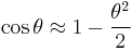
The small-angle approximation is a useful simplification of the basic trigonometric functions which is approximately true in the limit where the angle approaches zero. They are truncations of the Taylor series for the basic trigonometric functions to a second-order approximation. This truncation gives:

$\sin \theta \approx \theta$

$\cos \theta \approx 1 - \frac{\theta^2}{2}$

$\tan \theta \approx \theta$ ,

where θ is the angle in radians.

The small angle approximation is useful in many areas of physics, including mechanics, electromagnetics, optics (where it forms the basis of the paraxial approximation), cartography, astronomy, and so on.

1 Justifications
2 Error of the approximations
3 Specific uses
4 See also
5 References

Justifications

Graphic

The accuracy of the approximations can be seen below in Figure 1 and Figure 2. As the angle approaches zero, it is clear that the gap between the approximation and the original function quickly vanishes.

Geometric

The red section on the right, d, is the difference between the lengths of the hypotenuse, H, and the adjacent side, A. As is shown, H and A are almost the same length, meaning cos θ is close to 1 and $\theta^2/2$ helps to trim the red away.

$\cos{\theta} \approx 1 - \frac{\theta^2}{2}$

The opposite leg, O, is approximately equal to the length of the blue arc, s. Gathering facts from geometry, s = A*θ, from trigonometry, sin θ = O/H and tan θ = O/A, and from the picture, $O \approx s$ and $H \approx A$ leads to:

$\sin \theta = {O\over H}\approx{O\over A} = \tan \theta = {O\over A} \approx {s\over A} = {{A*\theta}\over A} = \theta$ .

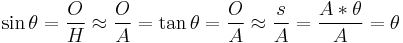Simplifying leaves,

$\sin \theta \approx \tan \theta \approx \theta$ .

Mathematical

The Taylor series about 0 of the trigonometric functions are^[1]

$\sin \theta = \sum^{\infin}_{n=0} \frac{(-1)^n}{(2n%2B1)!} x^{2n%2B1} = \theta - \frac{\theta^3}{3!} %2B \frac{\theta^5}{5!} - \frac{\theta^7}{7!} %2B \cdots$

$\cos \theta = \sum^{\infin}_{n=0} \frac{(-1)^n}{(2n)!} x^{2n} = 1 - \frac{\theta^2}{2!} %2B \frac{\theta^4}{4!} - \frac{\theta^6}{6!} %2B \cdots$

$\tan \theta = \sum^{\infin}_{n=1} \frac{B_{2n} (-4)^n (1-4^n)}{(2n)!} x^{2n-1} = \theta %2B \frac{\theta^3}{3} %2B \frac{2 \theta^5}{15} %2B \frac{17 \theta^7}{315} %2B \cdots$

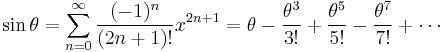
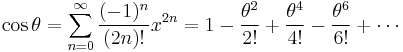
where θ is the angle and B_s are Bernoulli numbers.

When the angle θ is much less than one radian, its powers θ², θ³, ... decrease rapidly, so only a few are needed. The highest power included is called the order of the approximation. Neither sin θ nor tan θ has an θ² term, so their first- and second-order approximations are the same. Truncating the functions to the second order gives:

$\sin \theta \approx \theta$

$\cos \theta \approx 1 - \frac{\theta^2}{2}$

$\tan \theta \approx \theta$ .

Error of the approximations

Figure 3 shows the relative errors of the small angle approximations. The angles at which the relative error exceeds 1% are as follows:

tan θ ≈ θ at about 0.176 radians.
sin θ ≈ θ at about 0.244 radians.
cos θ ≈ 1 - θ²/2 at about 0.664 radians.

Specific uses

Astronomy

In astronomy, the angle subtended by the image of a distant object is often only a few arcseconds, so it is well suited to the small angle approximation. The linear size (D) is related to the angular size (X) and the distance from the observer (d) by the simple formula

D = X · d / 206,265

where X is measured in arcseconds.

The number 206,265 is approximately equal to the number of arcseconds in a circle (1,296,000), divided by 2π.

The exact formula is

D = d tan(X·2π/1,296,000)

and the above approximation follows when tan(X) is replaced by X.

Motion of a pendulum

The second order Cos approximation is especially useful in calculating the potential energy of a pendulum, which can then be applied with a Lagrangian to find the indirect (energy) equation of motion.

When calculating the period of a simple pendulum, the small-angle approximation for sine is used to allow the resulting differential equation to be solved easily by comparison with the differential equation describing simple harmonic motion.

Structural mechanics

The small angle approximation also appears in structural mechanics especially in stability and bifurcation analyses (mainly of axially-loaded columns ready to undergo buckling) leading to significant simplifications, though at a cost in accuracy and insight into the true behaviour.

Piloting

The 1 in 60 rule used in air navigation has its basis in the small-angle approximation, plus the fact that one radian is approximately 60 degrees.

References

^ Boas, Mary L. (2006). Mathematical Methods in the Physical Sciences. p. 26: Wiley. pp. 839. ISBN 978-0-471-19826-0.